LBM-Suite2p Quickstart#
Example Dataset
Example dataset collected by Kevin Barber with Dr. Alipasha Vaziri @ Rockefeller University.
Field |
Value |
|---|---|
Animal |
mk301 |
Date |
2025-03-01 |
Virus |
jGCaMP8s |
Framerate |
17 Hz |
FOV |
900 µm × 900 µm |
Resolution |
2 µm × 2 µm × 16 µm |
For installation with all gui/notebook dependencies, the following imports could take up to a minute depending on system resources.
from pathlib import Path
import matplotlib.pyplot as plt
import numpy as np
import suite2p
import mbo_utilities as mbo
import fastplotlib as fpl
import lbm_suite2p_python as lsp
See the assembly documentation for a guide on extracting data before input into suite2p.
Assembly TLDR
files = mbo.get_files("", "tif", 2)
scan = mbo.read_scan(r"D://demo//raw")
mbo.save_as(scan, "D://demo//assembled")
Suite2p is primarily a 2D pipeline - we will run each z-plane sequentially and combine results at the end.
Input data#
The tifs we use as input are planar timeseries [Txy].
Raw ScanImage tiffs will not work here, as they are not in the correct frame order.
mbo_utilities.get_metadata() will retrieve the ScanImage metadata (frame rate, pixel resolution, image dimensions). This happens internally in lbm_suite2p_python.run_plane() and lbm_suite2p_python.run_volume()}.
metadata = mbo.get_metadata(input_files[0])
ops = suite2p.default_ops()
ops = mbo.params_from_metadata(metadata, ops)

# we filled in pixel resolution and frame rate
ops["dx"], ops["dy"], ops["fs"]
lbm_suite2p_python.run_plane() will run with only a path to this file.
input_file = Path(input_files[7]) # pick a zplane in the middle of the cavity for example
input_file
If no save_path is given, it will save in the directory of your tiffs.
    This will create the following output directory structure

        /mnt/data/grid_search/
        ├── thr1.00_tau0.10/
        │   └── suite2p output for threshold_scaling=1.0, tau=0.1
        ├── thr1.00_tau0.15/
        ├── thr1.20_tau0.10/
        └── thr1.20_tau0.15/
Pick somewhere to save the results. For convenience, here we save to the same directory as this code is being run from.
save_path = Path("./results")
save_path.mkdir(exist_ok=True)
print(f"Saving suite2p results to:  {save_path.resolve()}")
Process a single z-plane#
ops = lsp.run_plane(
    ops=ops,
    input_tiff=input_file,
    save_path=save_path,
    save_folder = str(input_file.stem),  # strip the path and extension from this filename
    replot=True
)
Planar Outputs#
Previous users of Suite2p will regonize several files in their save_path::
ops.npy
stat.npy
spks.npy
iscell.npy
F.npy
Fneu.npy
Additionally, LBM-Suite2p-Python adds summary plots::
summary images (max-projection, mean-image)
Accepted/rejected masks drawn on summary image
20 randomly selected DF/F traces
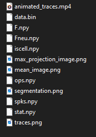
Note that depending on your suite2p I/O parameters, you may have a few additional files i.e. /reg_tif if you set ops["reg_tif"]=True.
Process full volume#
To run the entire volume, lbm_suite2p_python.run_volume() takes the same inputs as its planar variant, except give the full list of input files rather than a single input tiff file.
output_ops = lsp.run_volume(ops, input_files, save_path)
Once that is finished, we can use get_files to get a list of all ops.npy files.
ops_files = mbo.get_files(save_path.parent, 'ops', 8)
ops_files
Or all stat.npy files:
stat_files = mbo.get_files(save_path.parent, 'stat.npy', max_depth=5)
stat_files[:3]
Volumetric Outputs#
A few new files are now present at the root directory::
f_concat.npy: Volumetric version ofF.npyvolume_stats.npy: Contains signal quality, #accepted/rejected neurons for each Z-planemodel.npy: If you have rastermap installed, this is the rastermap outputF_embedding.npy: Another file used by rastermap
And a few new figures::
max_images_volume.mp4mean_images_volume.mp4segmentation_volume.mp4execution_time.pngmean_volume_signal.pngrastermap.png
Movies are essentially gifs that will play 1 z-plane per second.