Function Demos#
plot_traces#
lbm_suite2p_python.plot_traces()
plot_traces is a convenience function for plotting suite2p traces.
Data input is in the same format as F.npy: [n_neurons x n_timepoints].
For the most basic usage, simply pass in a loaded ops file or path to an ops file:
import lbm_suite2p_python as lsp
ops_file = lsp.load_ops("C://Users//RBO//lbm//Plane_07//plane0//ops.npy")
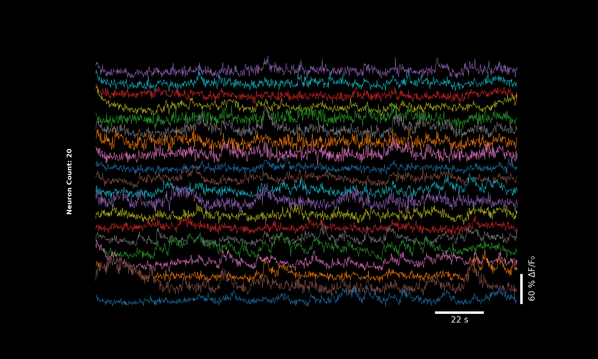
lsp.plot_traces(ops_file)
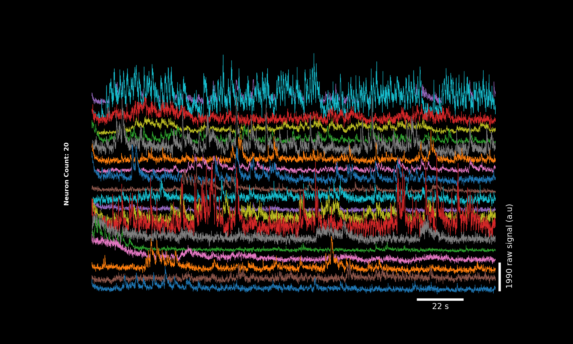
By default, plot_traces will plot 2 minutes of the \(\Delta F / F_0\) (%) for the first 20 neurons.
The \(\Delta F / F_0\) is calculated by calling dff_rolling_percentile().
The main features of this function:
automatic time and signal scalebars that adjust to the input data
automatic offset between traces calculated from the magnitude of the baseline signal
lower traces mask into upper traces to highlight the high-magnitude transients
from pathlib import Path
import mbo_utilities as mbo # for convenience
import lbm_suite2p_python as lsp
Gathering Data#
mbo_utilities.get_files()
lbm_suite2p_python.load_ops()
lbm_suite2p_python.load_traces()
This is a lazy way to get any ops.npy files in this directory.
ops_files = mbo.get_files(r"D:\W2_DATA", 'ops.npy', max_depth=10)
ops_files[:3]
We then use the ops.npy file to retrieve the traces:
ops = lsp.load_ops(ops_files[6])
f, fneu, spks = lsp.load_traces(ops) # only need f here
This f variable contains the loaded F.npy pre-filtered to only contain valid cells.
It can then be used to calculate \(\Delta F / F_0\)
dff = lsp.dff_percentile(f) * 100
Single neuron#
lsp.plot_traces(dff, './plot_traces_single.png', signal_units='dff', num_neurons=1)
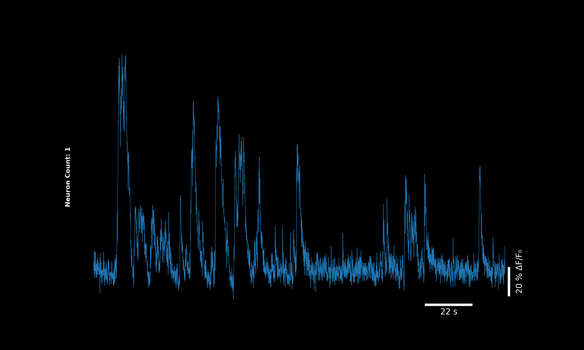
Single neuron trace (percentile-based DF/F).#
Two neurons#
lsp.plot_traces(dff, './plot_traces_double.png', signal_units='dff', num_neurons=2)
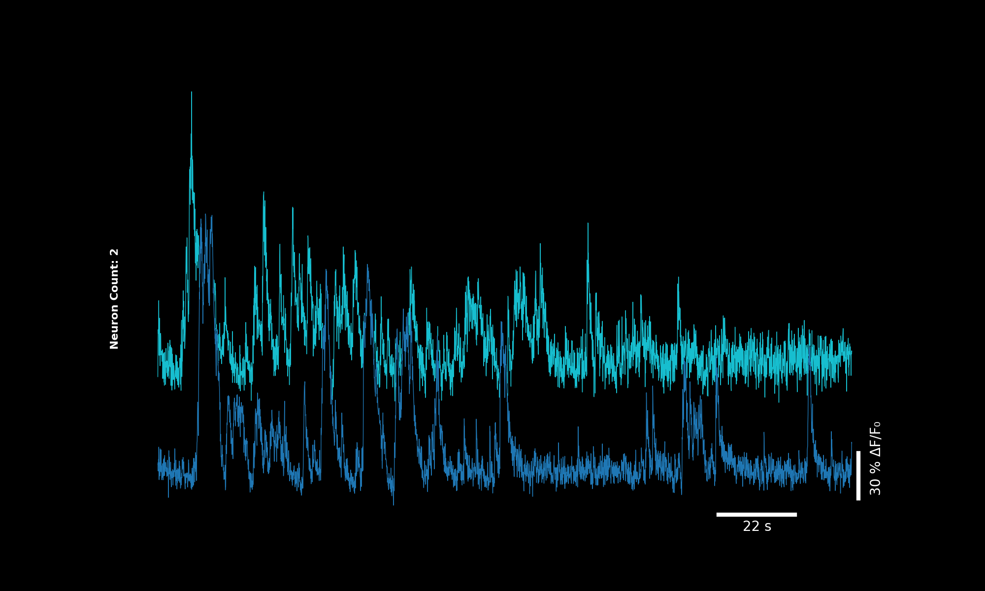
Two traces with offset autocalculated from baseline signal.#
Two neurons with manual offset#
lsp.plot_traces(dff, './plot_traces_single_gap50.png', signal_units='dff', num_neurons=2, offset=250)
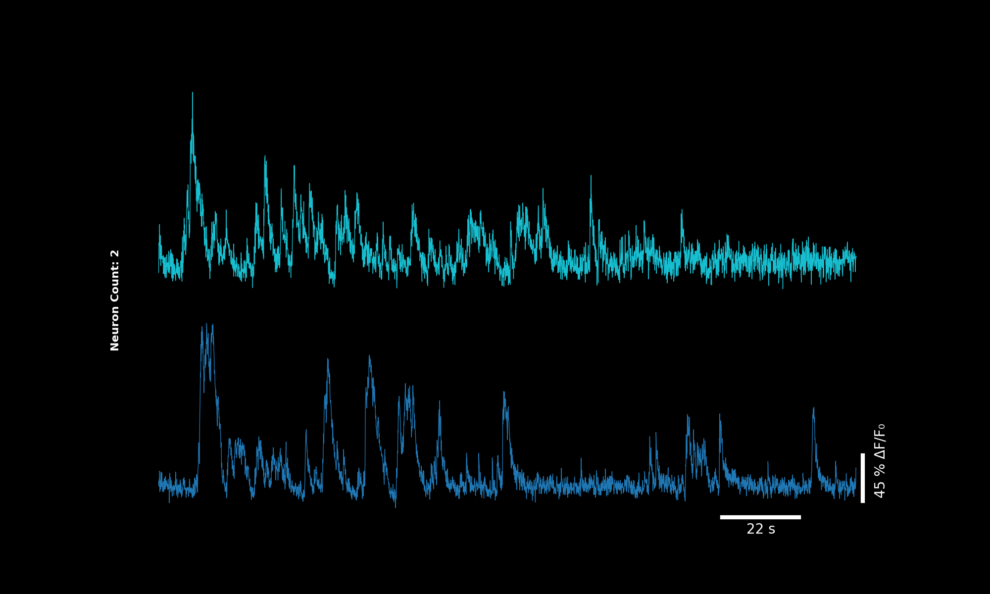
Two traces with manually specified offset.#
\(\Delta F / F_0\)#
lsp.plot_traces(dff, './plot_traces_dff.png', signal_units='dff')
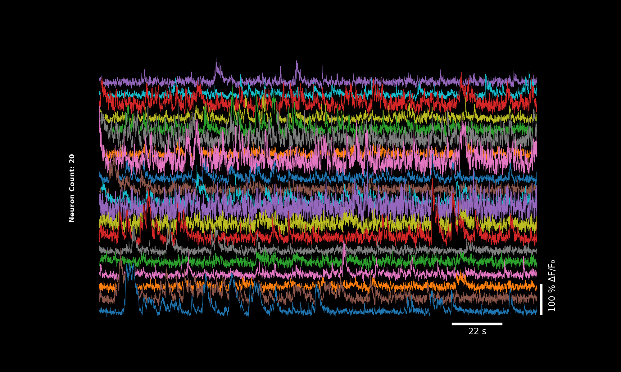
DFF is always shown in percentages.#
More neurons#
lsp.plot_traces(dff, './plot_traces_dff_50n.png', signal_units='dff', num_neurons=50)
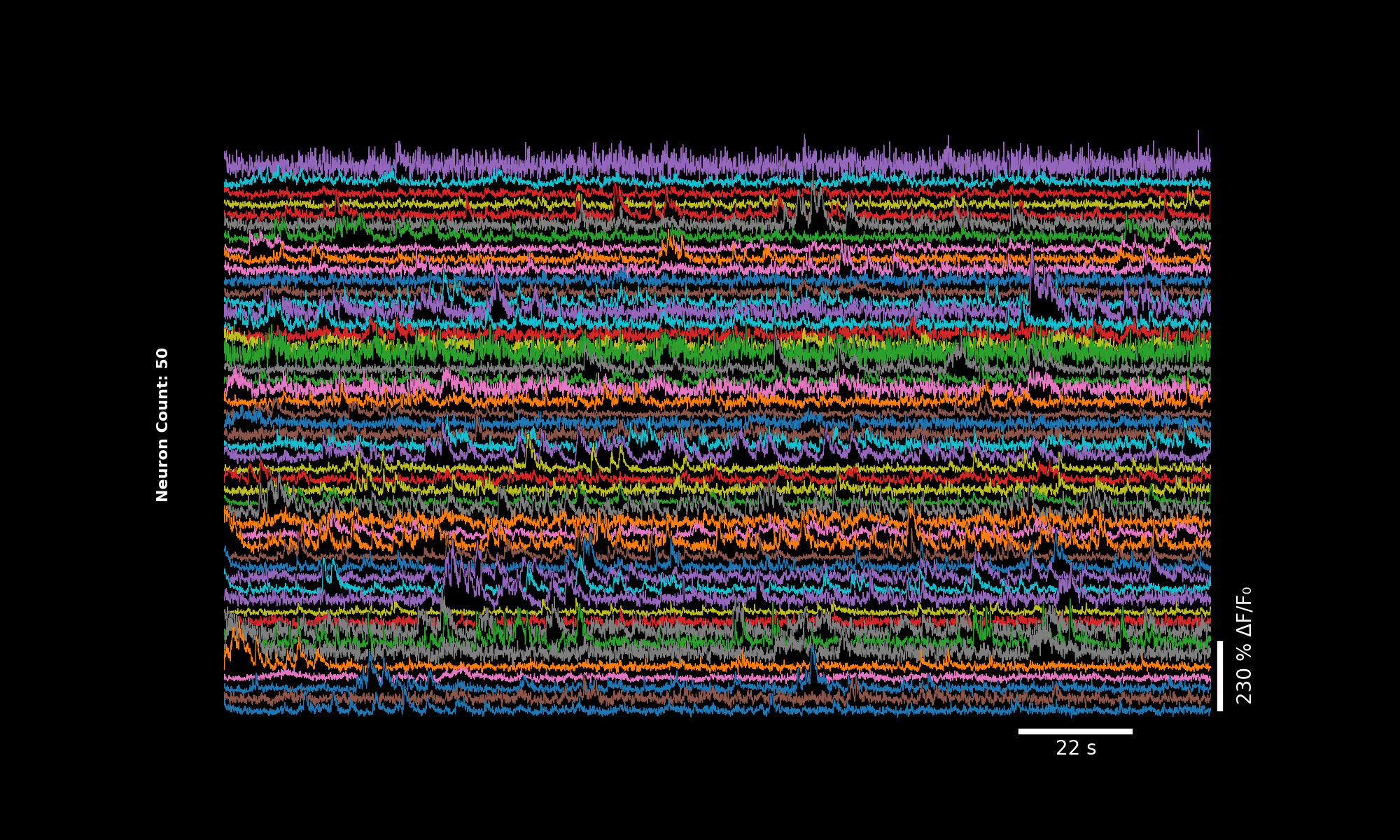
First 50 neurons, default colormap.#
100 neurons, custom colormap#
lsp.plot_traces(dff[::2], './plot_traces_dff_100n_nipy.png', signal_units='dff', num_neurons=100, cmap="nipy_spectral")
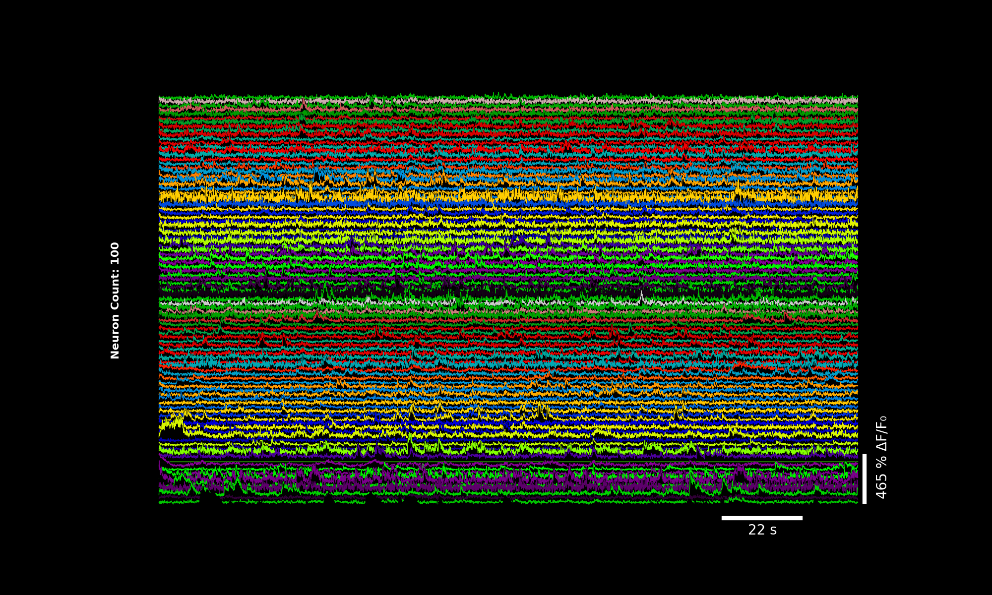
100 traces using the nipy_spectral colormap.#
Temporal binning#
2× binning#
bin_factor = 2
dff_binned = lsp.bin1d(dff, bin_factor)
fps_binned = metadata["frame_rate"] / bin_factor
lsp.plot_traces(dff_binned, './plot_traces_dff_binned_2x.png', signal_units='dff', fps=fps_binned)
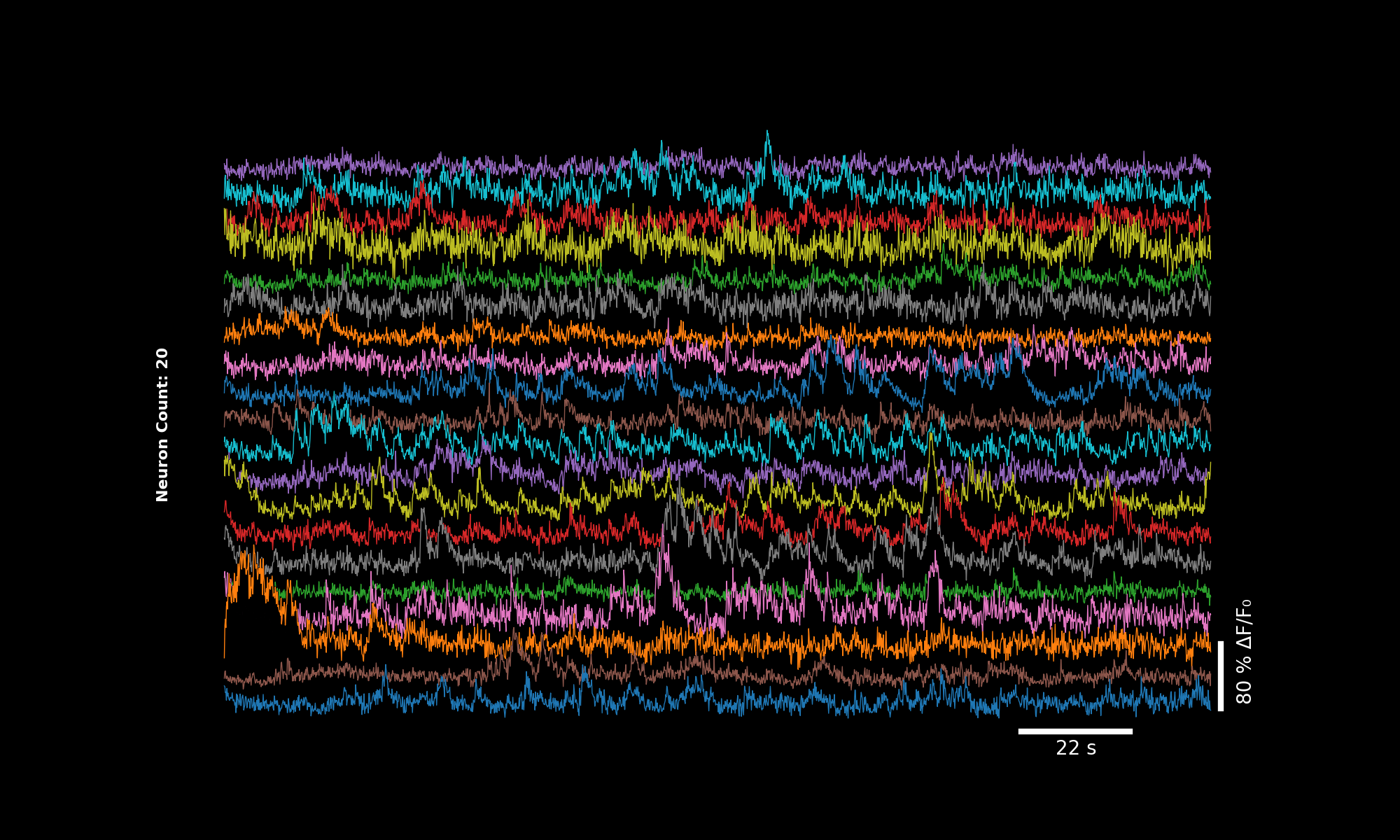
Traces downsampled by factor 2. Scale bar adjusts accordingly.#
4× binning#
bin_factor = 4
dff_binned_4x = lsp.bin1d(dff, bin_factor)
fps_binned_4x = metadata["frame_rate"] / bin_factor
lsp.plot_traces(dff_binned_4x, './plot_traces_dff_binned_4x.png', signal_units='dff', fps=fps_binned_4x)
Traces downsampled by factor 4. Horizontal scale bar still valid.#