1. Image Assembly#
Raw ScanImage .tiff files are saved to disk in an interleaved manner.
mbo_utilities.imread reads these files directly, returning a lazy array with shape [T, Z, Y, X] and ScanImage metadata attached. This replaces the previous scanreader-based workflow.
The general workflow is:
Set up filepaths.
Use
mbo_utilities.imreadto load raw.tifffiles as a lazy array.Optionally preview with
fastplotlib.Save assembled planes to disk with
mbo_utilities.save_as, or pass directly to the pipeline.
%load_ext autoreload
%autoreload 2

from pathlib import Path
import numpy as np

import fastplotlib as fpl
import matplotlib.pyplot as plt

from mbo_utilities import imread, get_files
import mbo_utilities as mbo
1.1. Input data: Path to your raw .tiff file(s)#
Before processing, ensure:
Put all raw
.tifffiles, from a single imaging session, into a directory.Here, we name that directory
raw
No other
.tifffiles reside in this directory
1.2. Load raw ScanImage data#
Pass a directory or file path to imread. It returns a lazy array with shape [T, Z, Y, X] and metadata from the ScanImage headers.
parent_dir = r"D:\SANDBOX\demo"
raw_tiff_files = get_files(parent_dir, str_contains='tif', max_depth=1)
raw_tiff_files
1.3. Lazy array#
imread returns a lazy array with shape [T, Z, Y, X]. Data is not loaded into memory until you index into it or call np.asarray().
The array carries ScanImage metadata as .metadata.
scan = imread(parent_dir)

print(f"Shape [T, Z, Y, X]: {scan.shape}")
print(f"Dtype: {scan.dtype}")

if hasattr(scan, "metadata"):
    meta = scan.metadata
    print(f"Frame rate: {meta.get('fr', 'N/A')} Hz")
    print(f"Num planes: {meta.get('num_planes', 'N/A')}")
preview_widget = fpl.ImageWidget(scan, histogram_widget=False, graphic_kwargs={"vmin": -300, "vmax": 12000})
preview_widget.show()
preview_widget.close()
nframes, nplanes = scan.shape[0], scan.shape[1]
print(f"Planes: {nplanes}")
print(f"Frames: {nframes}")
Lazy arrays support numpy-style indexing without loading everything into memory.
# single plane: [T, Y, X]
array = scan[:100, 0, :, :]
print(f"[T, Y, X]: {array.shape} (first 100 frames, plane 0)")
# multiple planes: [T, Z, Y, X]
array = scan[:100, 1:3, :, :]
print(f"[T, Z, Y, X]: {array.shape} (first 100 frames, planes 1-2)")
del array
1.3.1. View a single z-plane timeseries#
You can pass in the scan object to preview your data before saving it to disk.
Warning
Make sure you set histogram_widget=False or you will get an index error.
image_widget = fpl.ImageWidget(scan, histogram_widget=False,  figure_kwargs={"size": (900, 560)},graphic_kwargs={"vmin": -300,"vmax": 12000}))
image_widget.figure[0, 0].auto_scale()
image_widget.show()
image_widget.close()
1.3.2. Include more z-planes for a 4D graphic#
1.4. Path to save your files#
We can save the assembled planes to disk. The currently supported file extensions are .tiff.
You can also skip this step entirely and pass the lazy array directly to lcp.pipeline().
save_path = Path(parent_dir) / 'assembled'
save_path.mkdir(exist_ok=True)
We pass our scan object, along with the save path into mbo.save_as()
mbo.save_as(scan, save_path, overwrite=True, append_str="_assembled", ext='.tiff')
Reading tiff series data...
Reading tiff pages...
Raw tiff fully read.
Saving 14 planes.
Saving chunks: 100%|██████████████████████████████████████████████████████████████████████████████████████| 196/196 [00:06<00:00, 30.62it/s]
Data successfully saved to D:\SANDBOX\demo\assembled\plane_1_assembled.tiff.
Saving chunks: 100%|██████████████████████████████████████████████████████████████████████████████████████| 196/196 [00:06<00:00, 29.57it/s]
Data successfully saved to D:\SANDBOX\demo\assembled\plane_2_assembled.tiff.
Saving chunks: 100%|██████████████████████████████████████████████████████████████████████████████████████| 196/196 [00:06<00:00, 29.86it/s]
Data successfully saved to D:\SANDBOX\demo\assembled\plane_3_assembled.tiff.
Saving chunks: 100%|██████████████████████████████████████████████████████████████████████████████████████| 196/196 [00:06<00:00, 29.96it/s]
Data successfully saved to D:\SANDBOX\demo\assembled\plane_4_assembled.tiff.
Saving chunks: 100%|██████████████████████████████████████████████████████████████████████████████████████| 196/196 [00:06<00:00, 29.71it/s]
Data successfully saved to D:\SANDBOX\demo\assembled\plane_5_assembled.tiff.
Saving chunks: 100%|██████████████████████████████████████████████████████████████████████████████████████| 196/196 [00:06<00:00, 29.87it/s]
Data successfully saved to D:\SANDBOX\demo\assembled\plane_6_assembled.tiff.
Saving chunks: 100%|██████████████████████████████████████████████████████████████████████████████████████| 196/196 [00:06<00:00, 28.91it/s]
Data successfully saved to D:\SANDBOX\demo\assembled\plane_7_assembled.tiff.
Saving chunks: 100%|██████████████████████████████████████████████████████████████████████████████████████| 196/196 [00:06<00:00, 28.85it/s]
Data successfully saved to D:\SANDBOX\demo\assembled\plane_8_assembled.tiff.
Saving chunks: 100%|██████████████████████████████████████████████████████████████████████████████████████| 196/196 [00:06<00:00, 29.71it/s]
Data successfully saved to D:\SANDBOX\demo\assembled\plane_9_assembled.tiff.
Saving chunks: 100%|██████████████████████████████████████████████████████████████████████████████████████| 196/196 [00:06<00:00, 29.28it/s]
Data successfully saved to D:\SANDBOX\demo\assembled\plane_10_assembled.tiff.
Saving chunks: 100%|██████████████████████████████████████████████████████████████████████████████████████| 196/196 [00:06<00:00, 29.99it/s]
Data successfully saved to D:\SANDBOX\demo\assembled\plane_11_assembled.tiff.
Saving chunks: 100%|██████████████████████████████████████████████████████████████████████████████████████| 196/196 [00:06<00:00, 29.49it/s]
Data successfully saved to D:\SANDBOX\demo\assembled\plane_12_assembled.tiff.
Saving chunks: 100%|██████████████████████████████████████████████████████████████████████████████████████| 196/196 [00:06<00:00, 30.03it/s]
Data successfully saved to D:\SANDBOX\demo\assembled\plane_13_assembled.tiff.
Saving chunks: 100%|██████████████████████████████████████████████████████████████████████████████████████| 196/196 [00:06<00:00, 30.81it/s]
Data successfully saved to D:\SANDBOX\demo\assembled\plane_14_assembled.tiff.
Saving planes: 100%|████████████████████████████████████████████████████████████████████████████████████████| 14/14 [01:32<00:00, 6.59s/it]
Data successfully saved to D:\SANDBOX\demo\assembled.
1.4.1. Read back in your file to make sure it saved properly#
Make sure you include the append_str from the save_as() function.
img = imread(Path(save_path) / 'plane_1_assembled.tiff')
img.shape
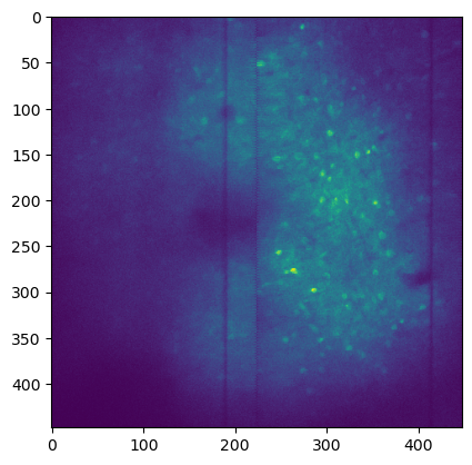
plt.imshow(np.mean(img,axis=0))
<matplotlib.image.AxesImage at 0x1f6d129a950>
image_widget = fpl.ImageWidget(img, figure_kwargs={"size":(1200, 800)})
image_widget.show()
image_widget.close()
1.4.2. Preview raw traces#
We can also preview the raw traces of the assembled image.
Click on a pixel to view the raw trace for that pixel over time.
from ipywidgets import VBox
iw_movie = fpl.ImageWidget(img, cmap="viridis", figure_kwargs={"size": (900, 560)},)

tfig = fpl.Figure()

raw_trace = tfig[0, 0].add_line(np.zeros(img.shape[0]))

@iw_movie.managed_graphics[0].add_event_handler("click")
def pixel_clicked(ev):
    col, row = ev.pick_info["index"]
    raw_trace.data[:, 1] =  iw_movie.data[0][:, row, col]
    tfig[0, 0].auto_scale(maintain_aspect=False)

VBox([iw_movie.show(), tfig.show()])