2. Explained: Source Extraction#
This section details background information helpful with Step 3: Segmentation
Source extraction is the umbrella term for a sequence of steps designed to distinguish neurons from background signal calculate the properties and characteristics of these neurons relative to the background.
The first step to source extraction is often the most computationally expensive step of calcium imaging pipelines: Segmentation.
Segmentation is the process of distinguishing between two spatially or temporally correlated neurons using object boundries and regions.
Subsequent processing would then involve cell identification, classification (assign labels), and extraction.
This pipeline centers around the segmentation algorithm Constrained Non-Negative Matrix Factorization (CNMF)
2.1. Constrained Non-Negative Matrix Factorization (CNMF)#
At a high-level, the CNMF algorithm works by:
Breaking the full FOV into patches of
patch_sizewith a setoverlapin each direction.Looking for
Knumber of components in each patch.Filter false positives.
Combine resulting neuron coordinates (spatial components) for each patch into a single structure:
A_keepandC_keep.The time traces (temporal components) in the original resolution are computed from
A_keepandC_keep.Detrended DF/F values are computed.
These detrended values are deconvolved.
2.2. Deconvolution#
The CNMF output yields “raw” traces, we need to deconvolve these to convert these raw traces to interpritable neuronal traces.
These raw traces are noisy, jagged, and must be denoised, detrended and deconvolved.
Note
Deconvolution and correlation metrics are closely related (see here for a helpful discussion).
Each raw trace is deconvolved via “constrained foopsi”, which yields:
g
: The decay (and for p=2, rise) coefficients.
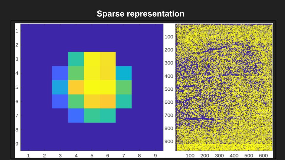
S
: The vector of “spiking” activity that best explain the raw trace.
Note
S should ideally be ~90% zeros, also known as “sparse”
S and g are then used to produce C (deconvolved traces), which looks like the raw trace Y, but much cleaner and smoother.
Important
The optional output YrA is equal to Y-C, representing the original raw trace.
2.3. Validating Neurons and Traces#
Note
Although it is important to understand the process governing validating neurons, this process is fully performed for you with no extra steps needed.
The key idea for validating our neurons is that we know how long the brightness indicating neurons activity should stay bright as a function of the number of frames.
That is, our calcium indicator (in this example: GCaMP-6s):
rise-time of 250ms
decay-time of 500ms
total transient time = 750ms
Frame rate = 4.7Hz
\(4.7Hz * (0.2 + 0.55) = 3\) frames per transient.
And thus the general process of validating neuronal components is as follows:
Use the decay time (0.5s) multiplied by the number of frames to estimate the number of samples expected in the movie.
Calculate the likelihood of an unexpected event (e.g., a spike) and return a value metric for the quality of the components.
Normal Cumulative Distribution function, input = -min_SNR.
Evaluate the likelihood of observing traces given the distribution of noise.