mbo_utilities: User Guide#
Installation | Supported Formats | MBO Hub
An image I/O library with an intuitive GUI for scientific imaging data.
Reading and Writing Data#
imread is a lazy-file reader.
Pass a file, list of files, or directory and it will read the image data and metadata.
Wrap a numpy array with imread(array) and have access to all lazy operations.
Volumetric data are read by passing in the directory containing each z-plane.
# Read any supported format - returns a lazy array
arr = mbo.imread(
    inputs,                      # Path, list of paths, directory, or numpy array
    # ScanImage TIFF options ---
    roi=None,                    # ROI selection: None=stitch, 0=split, N=specific ROI
    fix_phase=True,              # Enable bidirectional scan-phase correction
    phasecorr_method="mean",     # Phase estimation: "mean", "median", or "max"
    use_fft=False,               # Use FFT-based subpixel correction (slower, more precise)
    upsample=5,                  # Upsampling factor for subpixel phase estimation
    border=3,                    # Border pixels to exclude from phase calculation
    max_offset=4,                # Maximum phase offset to search (pixels)
    **kwargs                     # Additional format-specific options
)

# Write to any supported format
mbo.imwrite(
    lazy_array,                  # Source array (from imread or np.ndarray wrapped)
    outpath,                     # Output directory or file path
    ext=".tiff",                 # Output format: ".tiff", ".zarr", ".h5", ".bin", ".npy"
    planes=None,                 # Z-planes to export (1-based): None=all, int, or list
    frames=None,                 # Timepoints to export (1-based): None=all, int, or list
    channels=None,               # Channels to export (1-based): None=all, int, or list
    num_frames=None,             # Number of frames to write (None=all)
    roi_mode="concat_y",         # ROI handling: "concat_y" (stitch) or "separate"
    roi=None,                    # Specific ROI(s) when roi_mode="separate"
    register_z=False,            # Compute + apply axial plane-to-plane shifts
    metadata=None,               # Additional metadata dict to embed
    overwrite=False,             # Overwrite existing files
    order=None,                  # Reorder planes before writing
    target_chunk_mb=100,         # Target chunk size in MB for streaming
    output_name=None,            # Custom filename for .bin output
    output_suffix=None,          # Custom filename suffix (default: none)
    dataset_name=None,           # Dataset name for .h5 output
    dim_order=None,              # Axis labels for in-memory numpy arrays (e.g. "TZYX")
    progress_callback=None,      # Callback: func(progress, current_plane)
    show_progress=True,          # Show tqdm progress bar
    debug=False,                 # Enable verbose logging
    # Zarr-specific options (ext=".zarr") ---
    sharded=True,                # Use sharding (recommended for large data)
    ome=True,                    # Write OME-NGFF metadata
    compressor="none",           # "none", "gzip", "zstd", "blosc-lz4", "blosc-zstd"
    compression_level=1,         # compressor-specific level (gzip 0-9, zstd 1-22, blosc 1-9)
    pyramid=False,               # Generate multi-resolution pyramid
    pyramid_max_layers=4,        # Max pyramid resolution levels
    pyramid_method="mean",       # Pyramid downsampling method
    **kwargs                     # Additional format-specific options
)
from pathlib import Path
import numpy as np
import mbo_utilities as mbo
import matplotlib.pyplot as plt

RAW_PATH = Path(r"D:/demo/raw")
SAVE_PATH = RAW_PATH.parent / "corrected"
Load a data file#
This demo will use raw ScanImage tiffs.
Raw ScanImage TIFFs are detected automatically and return an MboRawArray:
help(mbo.imread)
arr = mbo.imread(RAW_PATH)

print(f"Type: {type(arr).__name__}")
print(f"Shape (T, C, Z, Y, X): {arr.shape}")
print(f"Planes: {arr.num_planes}, Frames: {arr.num_frames}, ScanImage multi-ROIs: {arr.num_rois}")
Type: LBMArray
Shape (T, C, Z, Y, X): (1574, 1, 14, 550, 448)
Planes: 14, Frames: 1574, ScanImage multi-ROIs: 2
Save a small test dataset#
Extract 100 frames from planes 7-9 to work with.
By default the filename is built from dimension tags only; pass output_suffix to append a custom suffix:
# arr.fix_phase = True  # Enable scan-phase correction
# arr.roi = None        # Stitch ROIs together

saved = mbo.imwrite(
    arr,
    SAVE_PATH,
    ext=".zarr",
    planes=[7, 8, 9],
    # num_frames=100,
    overwrite=True,
    roi=None,                    # 0 to separate, None to stitch ROIs
    output_suffix="example",     # filename suffix -> ..._zplane07-09_example.zarr
)
print(f"Saved to: {saved}")
Saved to: D:\demo\corrected
Read and explore the saved data#
# read the saved volume
arr = mbo.imread(saved)
print(f"Shape (T, C, Z, Y, X): {arr.shape}, Dtype: {arr.dtype}")
Shape (T, C, Z, Y, X): (1574, 1, 3, 550, 448), Dtype: int16
# Numpy-like indexing
frame = arr[0, 0, 0]        # First frame (Y, X)
subset = arr[10:20]         # Frames 10-19
crop = arr[:100, 0, 0, 100:200, 100:200]  # Spatial crop (T, Y, X)

print(f"Single frame: {frame.shape}")
print(f"Subset: {subset.shape}")
print(f"Crop: {crop.shape}")
Single frame: (550, 448)
Subset: (10, 1, 3, 550, 448)
Crop: (100, 100, 100)
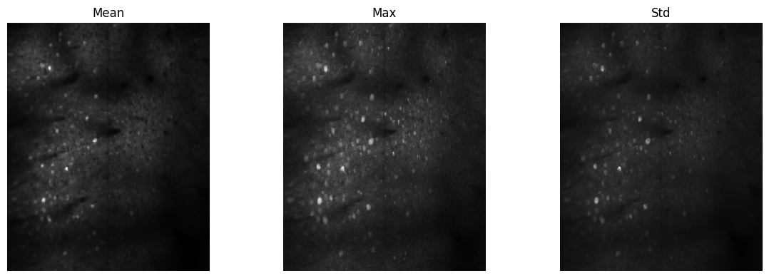
# Reduction operations
mean_img = arr[:200, 0, 0].mean(axis=0)
max_img = arr[:200, 0, 0].max(axis=0)
std_img = arr[:200, 0, 0].std(axis=0)

fig, axes = plt.subplots(1, 3, figsize=(12, 4))
axes[0].imshow(mean_img, cmap='gray'); axes[0].set_title('Mean')
axes[1].imshow(max_img, cmap='gray'); axes[1].set_title('Max')
axes[2].imshow(std_img, cmap='gray'); axes[2].set_title('Std')
for ax in axes: ax.axis('off')
plt.tight_layout()
plt.show()
Accessing metadata#
All lazy arrays expose metadata via the .metadata property:
metadata = arr.metadata
Imaging vs Acquisition Metadata#
Imaging metadata describes the physical data:
dx,dy,dz- voxel size in µmfs- frame rate in HzLx,Ly- image dimensions in pixelsnum_zplanes,num_timepoints,dtype
Acquisition metadata describes how the data was collected (ScanImage-specific):
num_mrois- number of scan regionsroi_groups,roi_heights- ROI configurationfix_phase,phasecorr_method- scan-phase correction settingszoom_factor,objective_resolution- optical parameters
Array-Type-Specific Metadata#
Some metadata only applies to certain stack types:
Parameter |
LBM Stack |
Piezo Stack |
Single Plane |
|---|---|---|---|
|
> 1 |
> 1 |
1 |
|
user-supplied |
from SI |
N/A |
|
no |
yes |
yes |
|
yes |
varies |
varies |
Quick Access#
View metadata via CLI:
uv run mbo info /path/to/data
uv run mbo /path/to/data --metadata
Planar vs Volumetric#
mbo_utilities infers volume structure from metadata and file layout:
Volumetric when
num_zplanes > 1,stack_typeislbm/piezo, or multipleplaneNN/Suite2p directories exist.Planar otherwise (a single plane, or a lone
ops.npy).
For Suite2p volumes each plane keeps its own ops.npy; the array’s top-level metadata mirrors plane 0 with num_zplanes set to the plane count.
Metadata when saving subsets#
Writing a subset (every Nth plane, a frame range) adjusts metadata automatically:
Selection |
Adjustment |
|---|---|
every Nth z-plane |
|
contiguous frame step |
|
non-contiguous frames |
|
from pprint import pprint
pprint(arr.metadata, depth=1)
{'C': 14,
 'ImageLength': 1116,
 'ImageWidth': 224,
 'LX': 224,
 'LY': 1116,
 'Lx': 448,
 'Ly': 550,
 'PhysicalSizeX': 2.0,
 'PhysicalSizeXUnit': 'micrometer',
 'PhysicalSizeY': 2.0,
 'PhysicalSizeYUnit': 'micrometer',
 'PhysicalSizeZ': None,
 'PhysicalSizeZUnit': 'micrometer',
 'T': 1574,
 'Z': 3,
 'apply_shift': False,
 'border': 3,
 'channels': 14,
 'color_channels': 1,
 'data_type': 'int16',
 'datatype': 'int16',
 'dims': [...],
 'dtype': dtype('<i2'),
 'dx': 2.0,
 'dy': 2.0,
 'dz': None,
 'file_paths': [...],
 'finterval': 0.07142857142857142,
 'fix_phase': True,
 'fov': [...],
 'fov_px': [...],
 'fov_um': [...],
 'fov_x': 224,
 'fov_y': 1116,
 'fps': 14.0,
 'fr': 14.0,
 'frameRate': 14.0,
 'frame_rate': 14.0,
 'frames_per_file': [...],
 'fs': 14.0,
 'height': 1116,
 'image_height': 1116,
 'image_width': 224,
 'is_contiguous': True,
 'is_lbm': True,
 'is_piezo': False,
 'lbmStack': True,
 'lbm_stack': True,
 'lx': 224,
 'ly': 1116,
 'max_offset': 4,
 'mean_subtraction': False,
 'n_channels': 14,
 'n_frames': 1574,
 'n_planes': 3,
 'n_rois': 2,
 'nc': 14,
 'nchannels': 14,
 'ncolors': 1,
 'ndim': 2,
 'nframes': 1574,
 'nplanes': 3,
 'nrois': 2,
 'nt': 1574,
 'numChannels': 14,
 'numPlanes': 14,
 'numROIs': 2,
 'num_channels': 3,
 'num_color_channels': 1,
 'num_colors': 1,
 'num_elements': 249984,
 'num_files': 2,
 'num_fly_to_lines': 16,
 'num_frames': 1574,
 'num_mrois': 2,
 'num_planes': 3,
 'num_px_x': 224,
 'num_px_y': 1116,
 'num_rois': 2,
 'num_timepoints': 1574,
 'num_z': 14,
 'num_zplanes': 3,
 'nx': 224,
 'ny': 1116,
 'nz': 3,
 'objective_resolution': 61,
 'offset': None,
 'ome': {...},
 'page_height': 1116,
 'page_width': 224,
 'phasecorr_method': 'mean',
 'piezoStack': False,
 'piezo_stack': False,
 'pixel_resolution': [...],
 'pixel_type': 'int16',
 'planes': 14,
 'roi': [...],
 'roi_groups': [...],
 'roi_heights': [...],
 'roi_mode': 'concat_y',
 'roi_px': [...],
 'roi_size': [...],
 'sampling_frequency': 14.0,
 'scanFrameRate': 14.0,
 'scanimage_multirois': 2,
 'shape': [...],
 'si': {...},
 'size': 249984,
 'size_x': 224,
 'size_y': 1116,
 'slices': 3,
 'stackType': 'lbm',
 'stack_type': 'lbm',
 'timepoints': 1574,
 'total_elements': 249984,
 'uniform_sampling': 1,
 'upsample': 5,
 'use_fft': True,
 'voxel_size': [...],
 'width': 224,
 'z_step': None,
 'zoom_factor': 2,
 'zplanes': 3}
Saving data: Formats and Conversions#
Convert between any supported formats with imwrite().
Here, we load the .zarr previously saved, add some metadata, and re-save to several of the supported formats.
Note: Keep different filetypes in separate directories.
Warning
When saving z-planes with inconsistent frame counts (e.g., some planes have 1574 frames, others have 1500), only the minimum number of frames across all planes will be written.
new_metadata = {"test": [123]}

# Each format takes its own array-specific options alongside `metadata`:
# zarr: storage layout (sharding + compression)
mbo.imwrite(arr, SAVE_PATH / "zarr", ext=".zarr", overwrite=True,
            metadata=new_metadata, sharded=True, compressor="zstd")
# tiff: no format-specific options
mbo.imwrite(arr, SAVE_PATH / "tiff", ext=".tiff", overwrite=True,
            metadata=new_metadata)
# h5: dataset name to write the volume under
mbo.imwrite(arr, SAVE_PATH / "hdf5", ext=".h5", overwrite=True,
            metadata=new_metadata, dataset_name="mov")
# suite2p .bin: needs the frame rate (fs) for ops.npy
mbo.imwrite(arr, SAVE_PATH / "suite2p", ext=".bin", overwrite=True,
            metadata={**new_metadata, "fs": 17.0})

print(f"New metadata: {mbo.imread(SAVE_PATH / 'tiff').metadata['test']}")
Working with In-Memory Numpy Arrays#
You can wrap any numpy array with imread() to get full imwrite() support, including zarr chunking, compression, and sharding.
For detailed documentation on NumpyArray properties, methods, and use cases, see Supported Formats.
import numpy as np
import mbo_utilities as mbo

data = np.random.randn(100, 512, 512).astype(np.float32)
np_out = RAW_PATH.parent / "test_numpy_array"

# Wrap with imread - returns a NumpyArray lazy array
arr = mbo.imread(data)
print(arr)  # NumpyArray(shape=(100, 1, 1, 512, 512), dtype=float32, dims='TCZYX' (in-memory))

# Now you can use imwrite with all features
mbo.imwrite(arr, np_out, ext=".zarr")   # Zarr with chunking/sharding
mbo.imwrite(arr, np_out, ext=".tiff")   # BigTIFF
mbo.imwrite(arr, np_out, ext=".bin", metadata={"fs": 14})    # Suite2p binary format
mbo.imwrite(arr, np_out, ext=".h5")     # HDF5

# 4D arrays (T, Z, Y, X) also work
volume = np.random.randn(100, 15, 512, 512).astype(np.float32)
arr4d = mbo.imread(volume)
print(f"dims: {arr4d.dims}, num_planes: {arr4d.num_planes}")  # dims: TCZYX, num_planes: 15

# Write specific planes (1-based indexing)
mbo.imwrite(arr4d, np_out, ext=".zarr", planes=[1, 8, 15])
User Interface: Miller Brain Studio#
The GUI can be launched in two ways:
From Python (Jupyter Lab or Jupyter Notebook only, not VSCode):
from mbo_utilities.gui import run_gui
run_gui(arr)
From the command line (works anywhere):
uv run mbo /path/to/data
See the GUI documentation for details.
# To run from the command line, through jupyter:
!uv run mbo --help
Usage: mbo [OPTIONS] COMMAND [ARGS]...

  MBO Utilities CLI - data preview and processing tools.

  GUI Mode:
    mbo                            Open file selection dialog
    mbo /path/to/data              Open specific file in GUI
    mbo /path/to/data --metadata   Show only metadata

  Commands:
    mbo init [DATA_PATH]           Create starter notebooks
    mbo convert INPUT OUTPUT       Convert between formats
    mbo info INPUT                 Show array information (CLI)
    mbo formats                    List supported formats

  Utilities:
    mbo --check-install                 Verify installation

Options:
  --check-install       Verify the installation of mbo_utilities and
                        dependencies.
  --help                Show this message and exit.

Commands:
  convert  Convert imaging data between formats.
  formats  List supported file formats.
  info     Show information about an imaging dataset.
  init     Create starter notebooks (mbo + LBM-Suite2p user guides).
  view     Open imaging data in the GUI viewer.
!uv run mbo info D:/demo/raw
Loading: D:/demo/raw

Array Information:
  Type:  MboRawArray
  Shape: (1574, 14, 550, 448)
  Dtype: int16
  Ndim:  4
  Files: 2
    - D:\demo\raw\demo_mk355_7_27_2025_00001.tif
    - D:\demo\raw\demo_mk355_7_27_2025_00002.tif

Metadata:
  nframes: 1574
  num_frames: 1574
  num_rois: 2
  ... and 42 more keys
Counting frames:   0%|          | 0/2 [00:00<?, ?it/s]
Counting frames: 100%|██████████| 2/2 [00:00<?, ?it/s]
Special array characteristics#
Lazy arrays have special characteristics depending on what the filetype is used for.
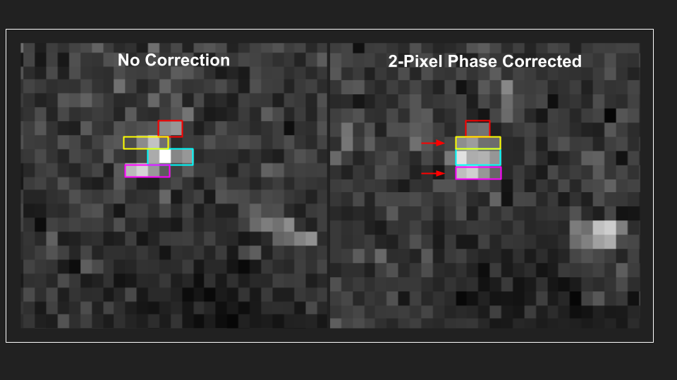
Bi-directional Scan-phase correction (ScanImage Tiff)#
ScanImage Tiffs (MboRawArray) only.
Bidirectional scanning creates phase offsets between alternating lines:
arr = mbo.imread(RAW_PATH)
arr.roi = None
z = 13  # plane with the largest residual scan-phase offset in this dataset

# scan-phase correction OFF: raw frames as acquired
arr.fix_phase = False
raw = arr[:, 0, z].mean(axis=0)

# scan-phase correction ON, subpixel (FFT) so a sub-pixel shift is actually applied
# (use_fft=False rounds to whole pixels, so offsets < 0.5 px become a no-op)
arr.fix_phase = True
arr.use_fft = True
cor = arr[:, 0, z].mean(axis=0)
print(f"detected scan-phase offset: {arr.offset:.2f} px (subpixel)")

# zoom to a central window so the per-row shift is easier to see
h, w = raw.shape
crop = (slice(h // 2 - 60, h // 2 + 60), slice(w // 2 - 90, w // 2 + 90))

fig, axes = plt.subplots(1, 3, figsize=(15, 5))
axes[0].imshow(raw[crop], cmap="gray")
axes[0].set_title("No correction (raw)", fontsize=12, fontweight="bold")
axes[1].imshow(cor[crop], cmap="gray")
axes[1].set_title(f"Corrected ({arr.offset:.2f} px, subpixel)", fontsize=12, fontweight="bold")
axes[2].imshow((cor - raw)[crop], cmap="bwr")
axes[2].set_title("Difference (corrected - raw)", fontsize=12, fontweight="bold")
for a in axes:
    a.axis("off")
plt.tight_layout()
plt.show()
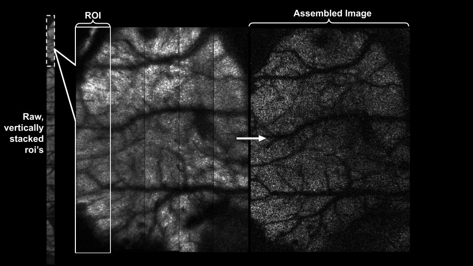
Multi-ROI handling (ScanImage Tiff)#
Control how multiple ROIs are handled.
By default, they are stitched horizontally:
arr = mbo.imread(RAW_PATH)
print(f"ROIs: {arr.num_rois}")

# roi=None: Stitch horizontally (default)
arr.roi = None
print(f"Stitched shape: {arr[0, 0, 7].shape}")

# roi=N: select a specific ROI (1-indexed)
arr.roi = 1
print(f"ROI 1 shape: {arr[0, 0, 7].shape}")
arr.roi = 2
print(f"ROI 2 shape: {arr[0, 0, 7].shape}")
ROIs: 2
Stitched shape: (550, 448)
ROI 1 shape: (550, 224)
ROI 2 shape: (550, 224)
Axial registration (plane-to-plane phase correlation)#
Light-beads-microscopy acquisition typically results in each z-plane having a spatial shift relative to adjacent planes. This can be corrected automatically by setting register_z=True.
Shifts are computed via phase correlation on a time-averaged mean image and stored in the array metadata as plane_shifts. They are not baked into the saved pixels — the raw data stays unshifted. Apply or remove them non-destructively at read time with with_axial_shifts (below). GPU (cupy) is used automatically if available.
arr = mbo.imread(RAW_PATH)
arr.roi = None
arr.fix_phase = True

# register_z computes a (dy, dx) shift per plane and stores them in metadata.
# imwrite returns the path to the store it wrote -- read that back directly so a
# directory holding other exports is never picked up by mistake.
zreg_path = mbo.imwrite(
    arr,
    SAVE_PATH / "zreg",
    ext=".zarr",
    num_frames=100,
    overwrite=True,
    register_z=True,
)
print(f"Saved to: {zreg_path}")
# inspect the computed shifts stored in metadata
saved = mbo.imread(zreg_path)
shifts = np.asarray(saved.metadata.get("plane_shifts", []))
print(f"Plane shifts (Y, X):
{shifts}")
Compare aligned vs unaligned, then save#
with_axial_shifts(saved) wraps the array so the stored plane_shifts are applied lazily on read; the source is never modified, and .enabled toggles between aligned and raw. The animation below scrolls through Z with the planes unaligned (left) vs aligned (right) — the cyan crosshair stays fixed, so a feature drifts on the left but holds still on the right. Then the aligned volume is saved to zarr so it can be reopened in mbo studio.
import matplotlib.animation as animation
from IPython.display import HTML

aligned = mbo.with_axial_shifts(saved)
Z = aligned.shape[2]
pt, pb, pl, pr = aligned.padding

# per-plane time-mean for each state, computed one plane at a time (low memory)
aligned.enabled = True
amean = np.stack([aligned[:, 0, z].mean(axis=0) for z in range(Z)])      # (Z, Yc, Xc)
aligned.enabled = False
rmean = np.stack([aligned[:, 0, z].mean(axis=0) for z in range(Z)])      # (Z, Y, X)

# place the raw planes on the same padded canvas so both panels match in size
Y, X = rmean.shape[-2:]
Yc, Xc = amean.shape[-2:]
umean = np.zeros((Z, Yc, Xc), dtype=amean.dtype)
umean[:, pt:pt + Y, pl:pl + X] = rmean

vmin, vmax = float(amean.min()), float(np.percentile(amean, 99.5))
fig, (axL, axR) = plt.subplots(1, 2, figsize=(8, 4.5))
imL = axL.imshow(umean[0], cmap="gray", vmin=vmin, vmax=vmax)
imR = axR.imshow(amean[0], cmap="gray", vmin=vmin, vmax=vmax)
for ax, title in ((axL, "Unaligned"), (axR, "Aligned")):
    ax.axhline(Yc / 2, color="cyan", lw=0.6, alpha=0.6)
    ax.axvline(Xc / 2, color="cyan", lw=0.6, alpha=0.6)
    ax.set_title(title, fontweight="bold")
    ax.axis("off")
sup = fig.suptitle(f"plane 0 / {Z - 1}")

def _update(z):
    imL.set_data(umean[z])
    imR.set_data(amean[z])
    sup.set_text(f"plane {z} / {Z - 1}")
    return imL, imR, sup

ani = animation.FuncAnimation(fig, _update, frames=Z, interval=600, blit=False)
plt.close(fig)

gif_path = SAVE_PATH / "axial_alignment.gif"
try:
    ani.save(gif_path, writer=animation.PillowWriter(fps=2))
    print(f"saved {gif_path}")
except Exception as e:
    print(f"(gif not saved: {e})")
HTML(ani.to_jshtml())
# bake the alignment in and save to zarr (streamed, source untouched).
# metadata drops plane_shifts since the saved pixels are already aligned.
aligned.enabled = True
aligned_path = mbo.imwrite(aligned, SAVE_PATH / "zreg_aligned", ext=".zarr", overwrite=True)
print(f"Saved aligned volume to: {aligned_path}")

# read it back the same way mbo studio does
check = mbo.imread(aligned_path)
print(f"Reads back as {type(check).__name__}, shape {check.shape}")
print(f'Open in mbo studio:  mbo "{aligned_path}"')
Supplying your own shifts#
with_axial_shifts also takes shifts directly via plane_shifts= — one (dy, dx) row per z-plane, so its length must equal the array’s Z size (it is validated against the "Z" axis). Use this when shifts come from another source or are adjusted by hand.
Miller Brain Studio applies valid plane_shifts automatically on load, so a volume saved with register_z=True opens already aligned with no extra step.
# supply shifts manually: one (dy, dx) row per z-plane (length must equal Z)
nz = saved.shape[2]
custom_shifts = [[0, 0], [2, -1], [3, -2]][:nz]

manual = mbo.with_axial_shifts(saved, plane_shifts=custom_shifts)
print(f"applied {len(custom_shifts)} shifts -> padded shape {manual.shape}")

manual.enabled = False   # toggle back to the raw frames, same object
print(f"raw shape {manual.shape}")
Video Export#
Export calcium imaging data to video files for presentations and sharing with to_video.
from mbo_utilities import imread, to_video

arr = imread("data.tif")

# basic export
to_video(arr, "output.mp4")

# quick preview with speed factor (10x playback)
to_video(arr, "preview.mp4", speed_factor=10)

# high-quality export for presentations
to_video(
    arr,
    "movie.mp4",
    fps=30,
    speed_factor=5,
    temporal_smooth=3,  # reduce frame-to-frame flicker
    gamma=0.8,          # brighten midtones
    quality=10,         # highest quality
)
Parameters#
Parameter |
Default |
Description |
|---|---|---|
|
30 |
Base frame rate |
|
1.0 |
Playback speed multiplier |
|
None |
Z-plane to export (for 4D data) |
|
0 |
Rolling average window (frames) |
|
0 |
Gaussian blur sigma (pixels) |
|
1.0 |
Gamma correction (<1 = brighter) |
|
None |
Matplotlib colormap name |
|
9 |
Video quality (1-10) |
|
1.0 |
Percentile for auto min |
|
99.5 |
Percentile for auto max |
4D Data#
For 4D data (T, Z, Y, X), select which z-plane to export:
to_video(arr_4d, "plane5.mp4", plane=5)