Quantifying Cell Activity#
The gold-standard formula for measuring cellular activity is “Delta F over F₀”, or the change in fluorescence intensity normalized by the baseline activity:
Here, F₀ a user-defined baseline that may be static (e.g., median over all frames) or dynamically estimated using a rolling window.
This guide assumes you’ve read this scientifica article by Dr Peter Rupprecht at the University of Zurich.
\(\Delta F/F\) reflects intracellular calcium levels, but often in a nonlinear way
\(\Delta F/F\) was initially introduced for organic dye calcium indicators in the 1930s
GCaMP behaves differently due to its low baseline brightness and its nonlinearity
There is no single recipe on how to compute \(\Delta F/F\)
Computation of \(\Delta F/F\) must be adapted to cell types, activity patterns, and noise
Interpretation of \(\Delta F/F\) requires knowledge about indicators, cell types, and confounds
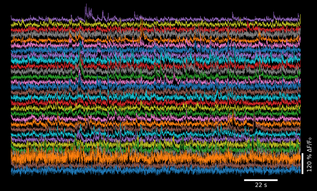
ΔF/F traces for 30 cells, sorted by similarity using the Rastermap algorithm.#
Indicator Dynamics#
Decay time constant (tau) per GCaMP variant — the fluorescence decay after a spike that deconvolution tools (Suite2p, OASIS/CNMF, CaImAn) take as a prior. Pick the value matching your indicator.
GCaMP Variant |
Optimal Tau (s) |
Notes / Sources |
|---|---|---|
GCaMP6f (fast) |
~0.5–0.7 s |
Suite2p: ~0.7 s (docs). OASIS/CNMF: ~0.5–0.7 s (PMC). CaImAn: ~0.4 s (docs). |
GCaMP6m (medium) |
~1.0–1.25 s |
Suite2p: ~1.0 s. OASIS: ~1.25 s (PMC). CaImAn: ~1.0 s (docs). |
GCaMP6s (slow) |
~1.5–2.0 s |
Suite2p: 1.25–1.5 s. OASIS/Suite2p: ~2.0 s (PMC). CaImAn: ~1.5–2.0 s. |
GCaMP7f (fast) |
~0.5 s |
Spike inference tuning (bioRxiv). Similar to GCaMP6f. |
GCaMP7m (medium) |
~1.0 s (est.) |
Estimated by analogy to GCaMP6m. No default in tools. |
GCaMP7s (slow) |
~1.0–1.5 s |
In vivo half-decay ~0.7 s (eLife). Tau ≈ 1.0 s. |
GCaMP8f (fast) |
~0.3 s |
OASIS fine-tuning (bioRxiv). Fastest decay; tenfold faster than 6f/7f (Nature). |
GCaMP8m (medium) |
~0.3 s |
|
GCaMP8s (slow) |
~0.7 s |
Spike inference optimal tau ~0.7 s (bioRxiv). Faster than 6s (Nature). |
Baseline F₀ Strategies#
Choosing the correct baseline strategy depends on many factors:
Cell type
Brain location
Frame-rate
Virus Kinetics
Scientific question
This table summarizes Calcium Activity detection strategies used in embryoinic development reviewed by Huang et al. [3].
Method |
How It’s Performed |
Pros |
Cons |
|---|---|---|---|
Percentile Baseline Subtraction |
Use a moving window to define F₀ as low percentile (e.g., 10–20th) of the trace. |
Adaptive baseline; handles long-term drift. |
Choice of window size/percentile affects sensitivity. |
Z-Score Thresholding |
Normalize trace by mean/SD, define events above N standard deviations. |
Removes baseline drift; good for noisy data. |
Sensitive to noise if SD is low; assumes Gaussian distribution. |
dF/F Thresholding |
Compute (F − F₀)/F₀ and define a fixed or adaptive threshold for events. |
Widely used; compatible with GCaMP, Fluo dyes. |
Sensitive to F₀ definition; arbitrary thresholds can bias results. |
Standard Deviation (SD) Masking |
Define active frames/regions where ΔF exceeds N×SD of baseline. |
Objective thresholding for event detection. |
Threshold choice heavily affects results. |
Image Subtraction (Frame-to-Frame) |
Compute ΔF = Fₙ − Fₙ₋₁ or F − background to detect sudden changes. |
Simple, fast; used for wave detection. |
Sensitive to noise; misses gradual changes. |
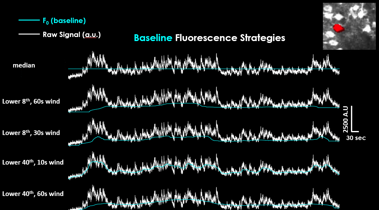
Comparison of different ΔF/F₀ baseline correction methods across selected cells.#
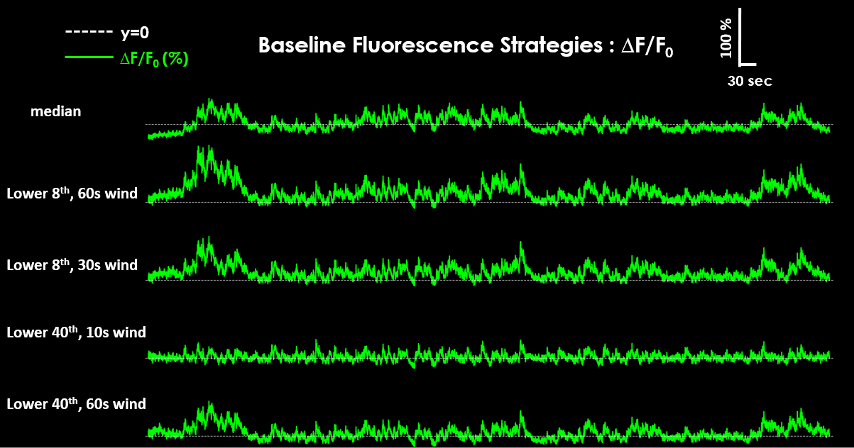
The resulting ΔF/F₀ traces can look different depending on the chosen baseline strategy.#
The resulting ΔF/F₀ traces can look different depending on the chosen baseline strategy.#
Standardized Noise Levels#
Compare shot-noise levels across datasets, recordings, experiments
Takes advantage of the slow calcium signal, which is typically similar between adjacent frames
Median to exclude outlies stemming from fast onset
Norm by sqrt(framerate) makes metric comparable across datasets with different framerates
Shot-noise decreases with #samples with a square root dependency
The resulting units, % for dF/F, divided by the square root of seconds, is strange.
This metric should be used relative to other datasets.
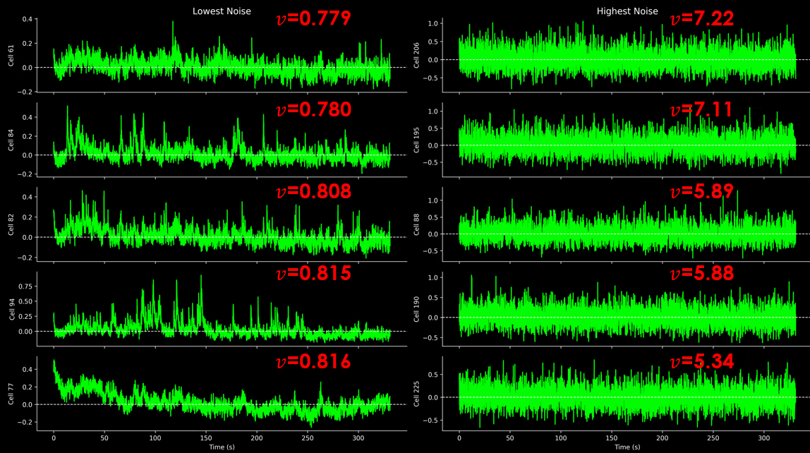
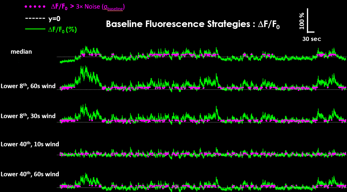
Top N neurons with highest and lowest standardized noise levels.#
Pipelines#
There are several pipelines for users to choose from when deciding how to process calcium imaging datasets. Often times, the outputs of these pipelines are in units that are not well documented. Even worse, the inputs to downstream pipelines pipelines require data to have particular units.
Example
This discussion, which details how to calculate noise for a variety of datasets, used traces that had the background signal subtracted.
This happens because CaImAn subtracts the background signal from each neuron under the hood. The resulting units are no longer raw signal, they are background-subtracted raw-signal. This process reduces the baseline F₀ to nearly zero and heavily skew ΔF/F₀ calculations.
CaImAn#
See: detrend_df_f
CaImAn computes ΔF/F₀ using a running low-percentile baseline.
By default, it uses the 8th percentile over a 500 frame window. The idea is to track the lower envelope of the signal to get F₀ without being biased by transients.
Neuropil/background: CaImAn handles this as part of its CNMF model [5].
Background and neuropil are explicitly separated into distinct spatial/temporal components, so the output traces are background subtracted during this matrix-factorization (as was the issue in the above example).
There is a strong argument to be made that a matrix factorization CNMF is not complex enough to model the true background and neuropil.
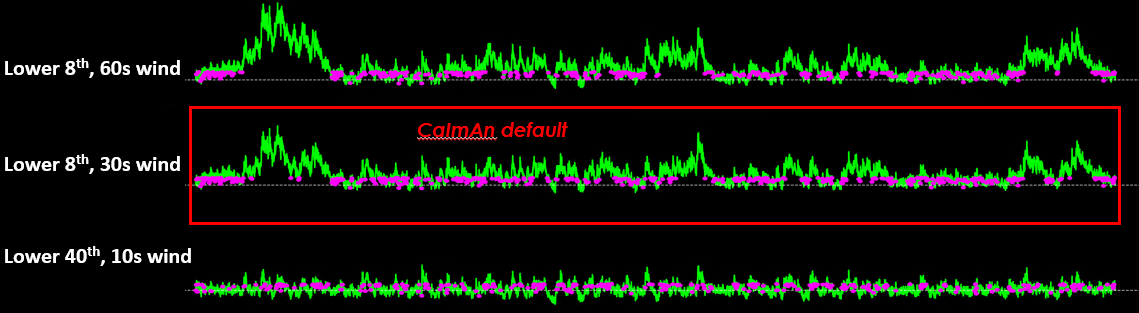
CaImAn uses a default baseline of the lower 8th percentile and a moving window of 200 frames.#
Giovannucci et al. [2]
Suite2p#
Suite2p does not output traces in ΔF/F₀ format directly.
Instead, it gives you the raw trace and the neuropil, along with spike estimates if you ran deconvolution. The neuropil represents fluorescence from the surrounding non-somatic tissue. As an optional step, many experimentors apply a fixed subtraction:
# F is an [n_neurons x time] array of raw signal
# Fneu is an [n_neurons x time] array of neuropil
F_corrected = F - 0.7 * Fneu
The 0.7 is an empirically chosen scalar to account for the partial contamination. Essentially you subtract 70% of the signal contained in the surrounding neuropil.
To compute ΔF/F₀, you divide trace, be that neuropil-corrected or not, by an F₀ you calculate yourself.
Internally, when running spike deconvolution, suite2p will convert your data into DF/F0 internally. For this, the default F₀ estimate comes from a “maximin” filter: smooth the trace with a Gaussian (default ~10 s), take a rolling min, then a max over a 60 s window.
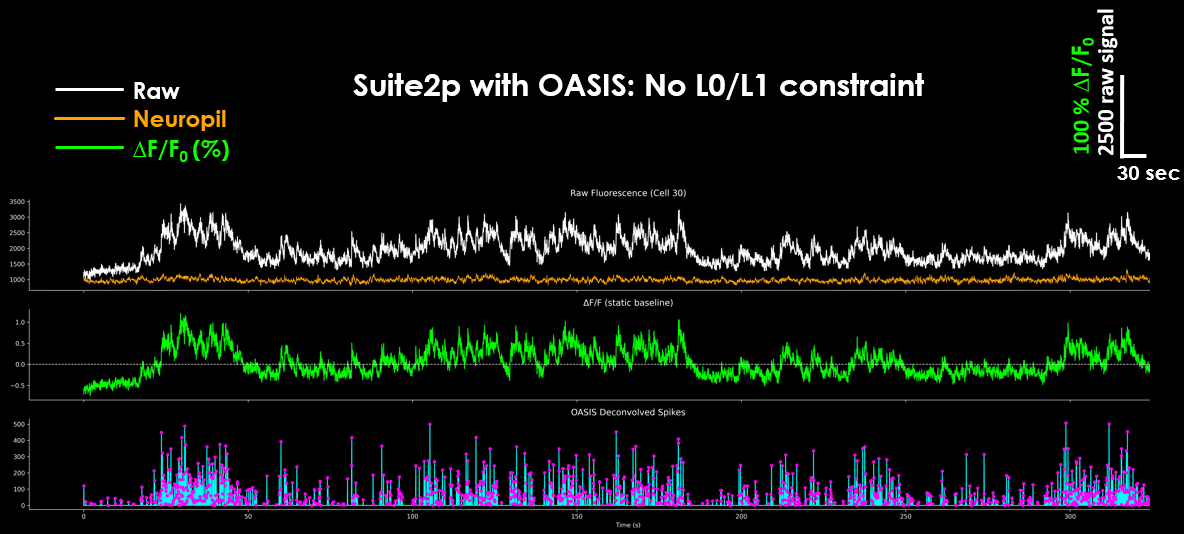
Raw, neuropil, ΔF/F₀ and resulting deconvolved spikes as output by Suite2p#
Pachitariu et al. [6]
EXTRACT#
EXTRACT outputs raw fluorescence signals without built-in ΔF/F₀ calculation. You compute it yourself using something like a low-percentile (e.g. 10%) as F₀. Most people use a global or sliding percentile window.
Neuropil: Handled implicitly. The algorithm uses robust factorization to ignore background and neuropil. There’s no explicit subtraction or coefficient to tune. It isolates only what fits a consistent spatial footprint and suppresses outliers by design.
Inan et al. [4], Dinç et al. [1]
Pipeline |
F₀ Method |
ΔF/F₀ |
Neuropil |
|---|---|---|---|
CaImAn |
8th percentile, 500-frame window |
Yes, in pipeline |
Modeled via CNMF, no manual subtraction |
Suite2p |
Maximin (default) or 8th percentile |
No, user divides post hoc |
0.7 × Fneu subtracted before baseline |
EXTRACT |
User-defined (e.g. 10th percentile) |
No, user computes |
Implicitly handled via robust model |
References#
Fatih Dinç, Hakan Inan, Oscar Hernandez, Claudia Schmuckermair, Omer Hazon, Tugce Tasci, Biafra O. Ahanonu, Yanping Zhang, Jérôme Lecoq, Simon Haziza, Mark J. Wagner, Murat A. Erdogdu, and Mark J. Schnitzer. Fast, scalable, and statistically robust cell extraction from large-scale neural calcium imaging datasets. bioRxiv, 2024. URL: https://www.biorxiv.org/content/10.1101/2021.03.24.436279, doi:10.1101/2021.03.24.436279.
Andrea Giovannucci, Johannes Friedrich, Pat Gunn, Jérémie Kalfon, Brandon L Brown, Sue Ann Koay, Jiannis Taxidis, Farzaneh Najafi, Jeffrey L Gauthier, Pengcheng Zhou, Baljit S Khakh, David W Tank, Dmitri B Chklovskii, and Eftychios A Pnevmatikakis. Caiman an open source tool for scalable calcium imaging data analysis. eLife, 8:e38173, 2019. URL: https://elifesciences.org/articles/38173, doi:10.7554/eLife.38173.
Lawrence Huang, Peter Ledochowitsch, Ulf Knoblich, Jérôme Lecoq, Gabe J Murphy, R Clay Reid, Saskia E J de Vries, Christof Koch, Hongkui Zeng, Michael A Buice, Jack Waters, and Lu Li. Relationship between simultaneously recorded spiking activity and fluorescence signal in gcamp6 transgenic mice. eLife, 10:e51675, 2021. URL: https://elifesciences.org/articles/51675, doi:10.7554/eLife.51675.
Hakan Inan, Murat A Erdogdu, and Mark Schnitzer. Robust estimation of neural signals in calcium imaging. In Advances in Neural Information Processing Systems, volume 30. Curran Associates, Inc., 2017. URL: https://proceedings.neurips.cc/paper/2017/hash/e449b9317dad920c0dd5ad0a2a2d5e49-Abstract.html.
Haifeng Liu, Zhaohui Wu, Xuelong Li, Deng Cai, and Thomas S. Huang. Constrained nonnegative matrix factorization for image representation. IEEE Transactions on Pattern Analysis and Machine Intelligence, 34(7):1299–1311, 2012. doi:10.1109/TPAMI.2011.217.
Marius Pachitariu, Carsen Stringer, Mario Dipoppa, Sylvia Schröder, L. Federico Rossi, Henry Dalgleish, Matteo Carandini, and Kenneth D. Harris. Suite2p: beyond 10,000 neurons with standard two-photon microscopy. bioRxiv, 2017. URL: https://www.biorxiv.org/content/10.1101/061507, doi:10.1101/061507.