Postprocessing Functions

This guide covers the postprocessing functions available in LBM-Suite2p-Python for analyzing and refining calcium imaging traces after Suite2p extraction.

ΔF/F Calculation

Rolling Percentile Baseline

The recommended method for computing ΔF/F₀ uses a rolling percentile baseline that adapts to slow drifts in fluorescence:

from lbm_suite2p_python import dff_rolling_percentile

# Basic usage
dff = dff_rolling_percentile(F, window_size=300, percentile=20)

# With auto-calculated window sizes based on indicator kinetics
dff = dff_rolling_percentile(
    F,
    tau=1.0,        # GCaMP decay constant (seconds)
    fs=30.0,        # Frame rate (Hz)
    percentile=20,  # Baseline percentile
)

Parameters:

• window_size: Rolling window in frames (~10 × tau × fs recommended)

• percentile: Percentile for baseline (20 is typical for calcium imaging)

• tau, fs: Auto-calculate window sizes from indicator kinetics

• smooth_window: Optional temporal smoothing (~0.5 × tau × fs)

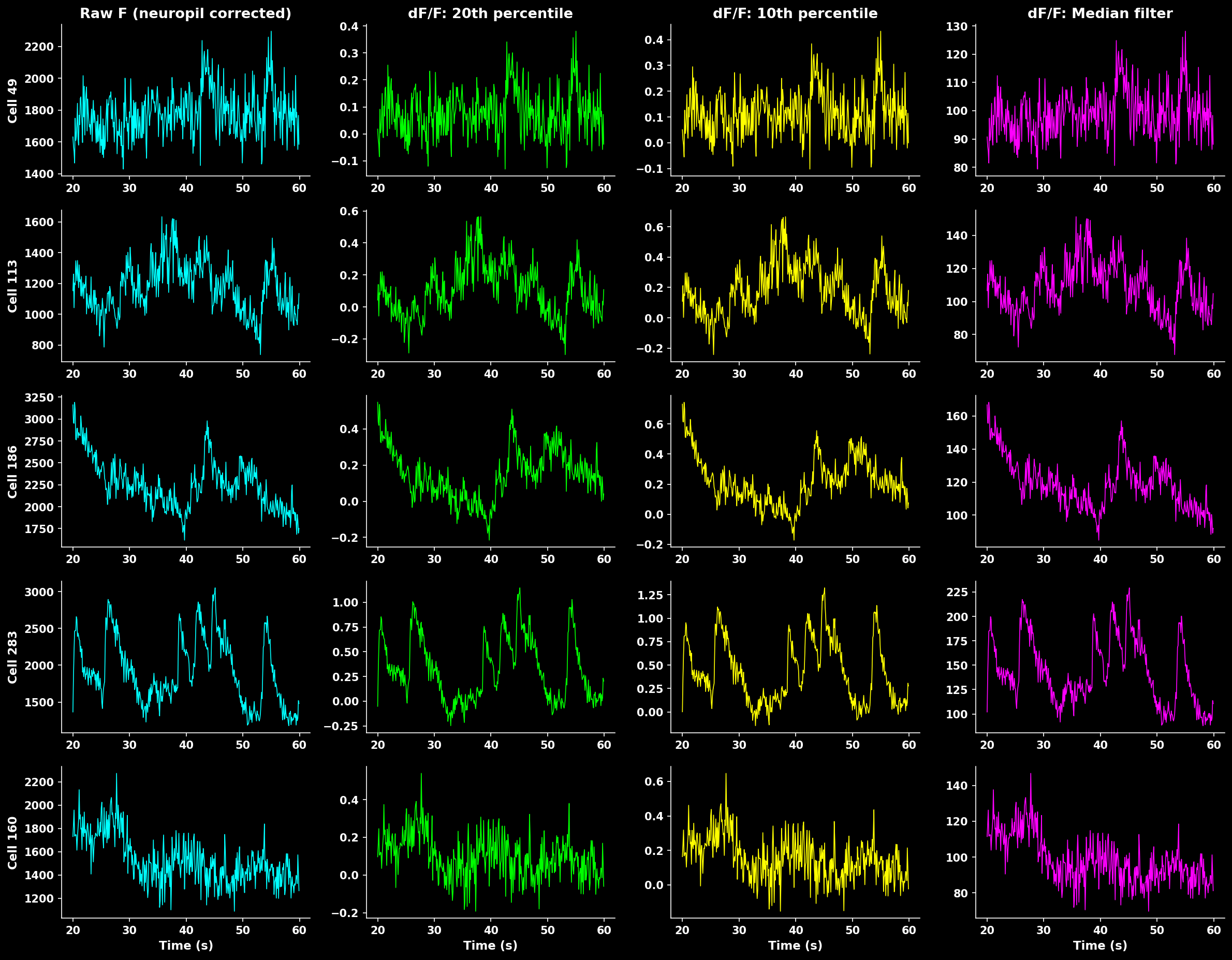
Comparison of different ΔF/F calculation methods. Rolling percentile (20th) provides robust baseline estimation that handles slow drifts while preserving transient peaks.

Window Size Effect

The window size critically affects baseline estimation:

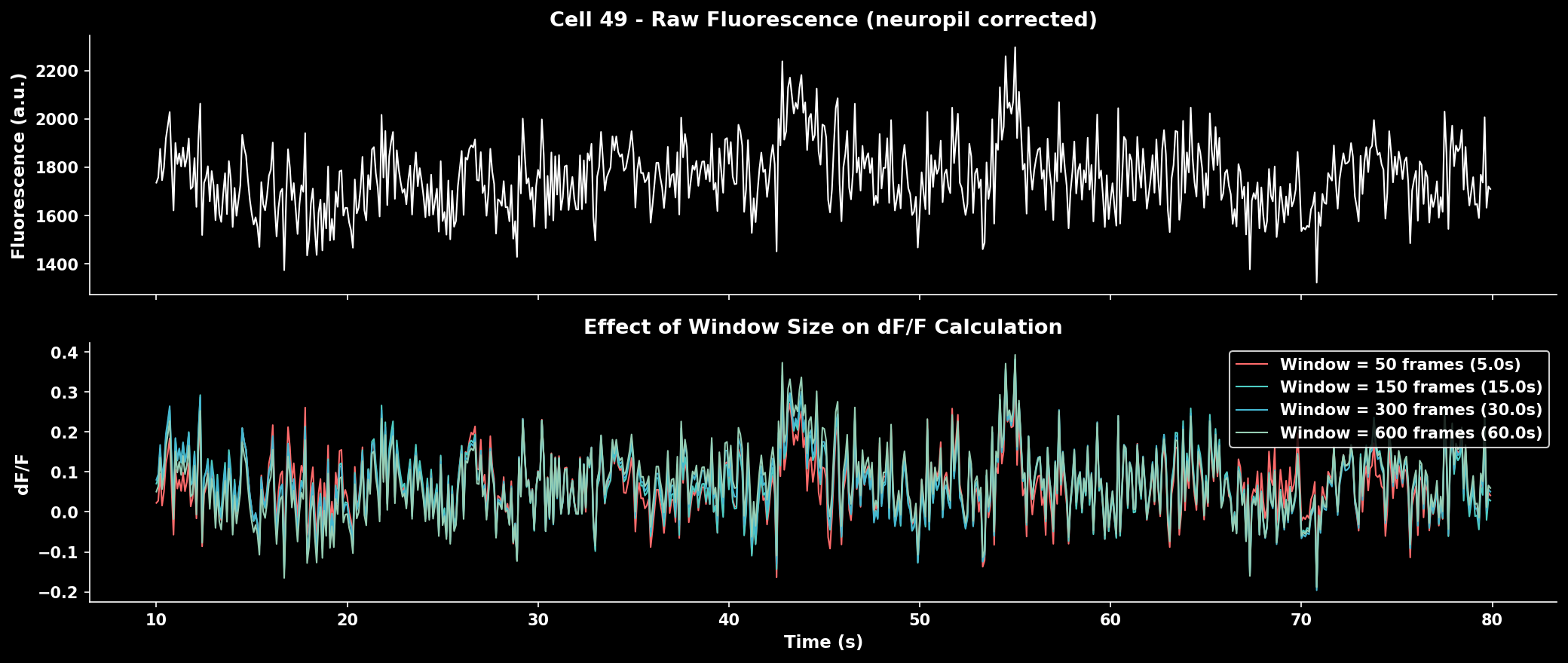
Effect of window size on ΔF/F calculation. Smaller windows track faster baseline changes but may contaminate baseline with transients. Larger windows provide stable baselines but miss slow drifts.

Rule of thumb: Use ~10× the indicator decay time constant (tau) × frame rate.

Indicator	Tau (s)	Frame Rate	Recommended Window
GCaMP6f	0.4	30 Hz	~120 frames
GCaMP6s	1.0	30 Hz	~300 frames
GCaMP7s	1.0	17 Hz	~170 frames
GCaMP8f	0.25	30 Hz	~75 frames

Median Filter Baseline

A simpler alternative for stable recordings:

from lbm_suite2p_python import dff_median_filter

dff = dff_median_filter(F)

Uses 1% of the median fluorescence as F₀. Fast but less adaptive to baseline drifts.

---

Noise Estimation

Shot Noise

Quantify recording quality using standardized shot noise levels:

from lbm_suite2p_python import dff_shot_noise

noise = dff_shot_noise(dff, fr=30.0)  # Returns noise in %/√Hz

The shot noise metric from Rupprecht et al. (2021) enables comparison across datasets:

\[\nu = \frac{\mathrm{median}_t\left( \left| \Delta F/F_{t+1} - \Delta F/F_t \right| \right)}{\sqrt{f_r}}\]

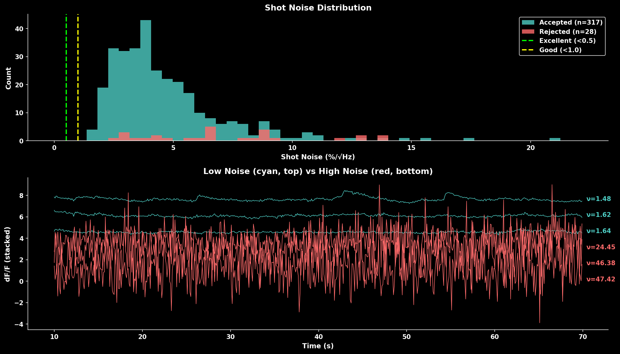
Shot noise distribution comparing accepted vs rejected cells. Lower noise indicates cleaner recordings. The trace panel shows example neurons with low noise (cyan, top) vs high noise (red, bottom).

Quality Benchmarks:

Noise Level	Quality	Interpretation
< 0.5 %/√Hz	Excellent	Very clean signal
0.5-1.0 %/√Hz	Good	Typical for healthy recordings
1.0-2.0 %/√Hz	Fair	May need filtering
> 2.0 %/√Hz	Poor	Consider excluding

---

Quality Scoring

Compute Trace Quality Score

Combine multiple metrics to rank neurons by signal quality:

from lbm_suite2p_python import compute_trace_quality_score

result = compute_trace_quality_score(
    F, Fneu, stat,
    fs=30.0,
    weights={'snr': 1.0, 'skewness': 0.8, 'shot_noise': 0.5}
)

# Access results
sorted_F = F[result['sort_idx']]  # Traces sorted best to worst
snr = result['snr']               # SNR values
scores = result['score']          # Combined scores

Metrics combined:

• SNR: Signal standard deviation / noise estimate (higher = better)

• Skewness: Positive skew indicates calcium transients (higher = better)

• Shot noise: Frame-to-frame variability (lower = better, inverted in score)

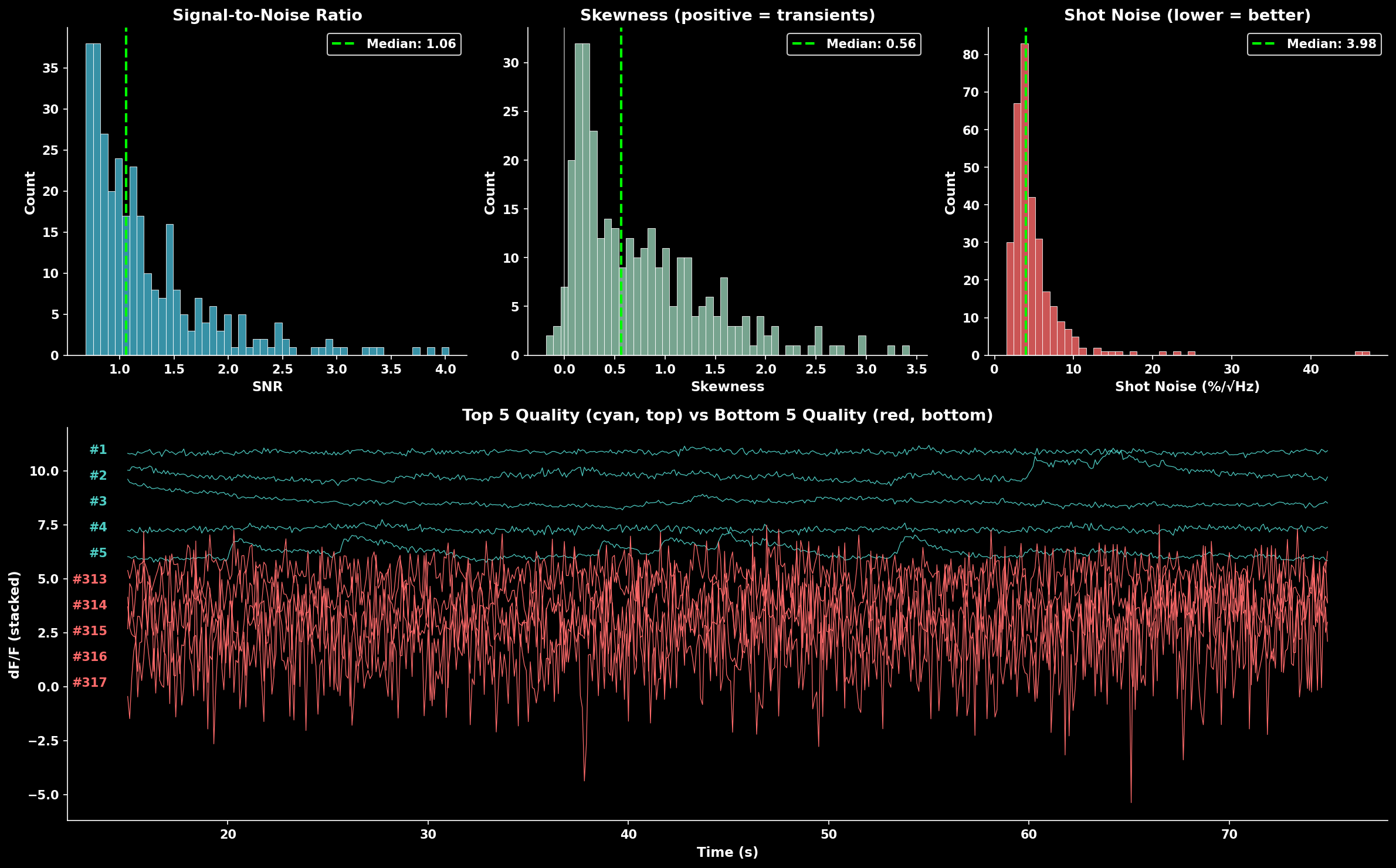
Quality score component distributions (SNR, skewness, shot noise) and example traces. The bottom panel shows top 5 quality neurons (cyan, top) vs bottom 5 quality neurons (red, bottom).

Sort Traces by Quality

Convenience function to sort traces:

from lbm_suite2p_python import sort_traces_by_quality

F_sorted, sort_idx, quality = sort_traces_by_quality(F, Fneu, stat, fs=30.0)

# Use sort_idx to sort other arrays
stat_sorted = stat[sort_idx]
iscell_sorted = iscell[sort_idx]

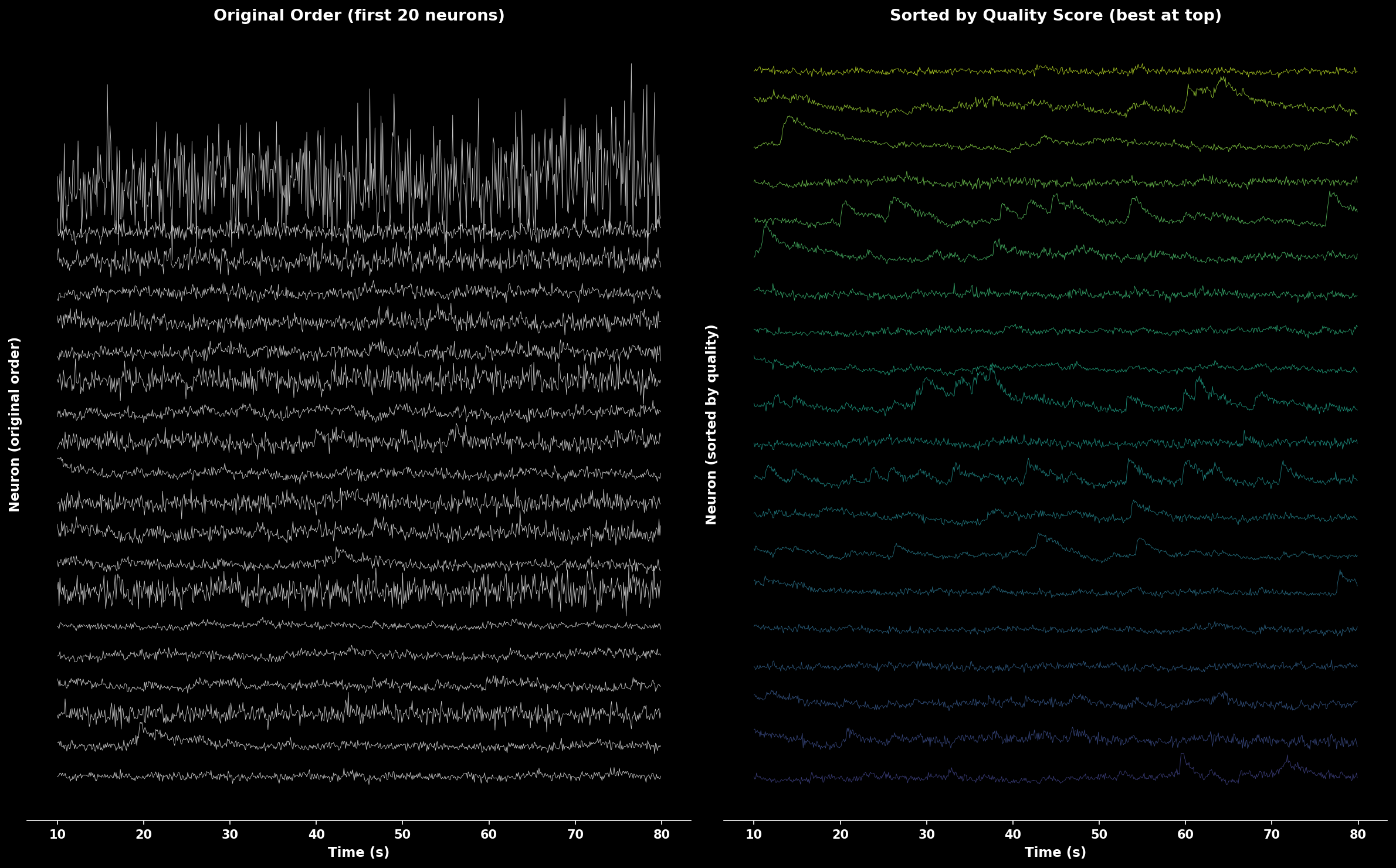
Comparison of traces in original order (left) vs sorted by quality score (right). Quality-sorted display shows best neurons at top with color gradient from high quality (yellow) to lower quality (purple).

---

Trace Normalization

Normalize Traces

Scale traces to [0, 1] range for visualization:

from lbm_suite2p_python.postprocessing import normalize_traces

# Min-max scaling per neuron
F_norm = normalize_traces(F, mode="per_neuron")

# Percentile-based scaling (more robust to outliers)
F_norm = normalize_traces(F, mode="percentile")

Comparison of normalization methods. Percentile-based scaling (1st-99th) is more robust to outliers than min-max scaling.

---

ROI Filtering

Filter by Diameter

Remove ROIs with abnormal sizes:

from lbm_suite2p_python.postprocessing import filter_by_diameter

iscell = filter_by_diameter(
    iscell, stat, ops,
    min_mult=0.3,  # Reject if < 30% of expected diameter
    max_mult=3.0   # Reject if > 300% of expected diameter
)

Filter by Area

Filter based on pixel count:

from lbm_suite2p_python.postprocessing import filter_by_area

iscell = filter_by_area(
    iscell, stat,
    min_mult=0.25,  # Reject if < 25% of median area
    max_mult=4.0    # Reject if > 400% of median area
)

Filter by Eccentricity

Remove elongated ROIs that are likely not cell bodies:

from lbm_suite2p_python.postprocessing import filter_by_eccentricity

iscell = filter_by_eccentricity(
    iscell, stat,
    max_ratio=5.0  # Reject if bounding box ratio > 5:1
)

Combined Filtering Example

from lbm_suite2p_python.postprocessing import (
    filter_by_diameter,
    filter_by_area,
    filter_by_eccentricity
)

# Load results
results = lsp.load_planar_results(ops_path)
iscell = results['iscell'][:, 0].astype(bool)
stat = results['stat']
ops = lsp.load_ops(ops_path)

# Apply filters sequentially
iscell = filter_by_diameter(iscell, stat, ops, min_mult=0.3, max_mult=3.0)
iscell = filter_by_area(iscell, stat, min_mult=0.25, max_mult=4.0)
iscell = filter_by_eccentricity(iscell, stat, max_ratio=5.0)

print(f"Accepted after filtering: {iscell.sum()}")

---

Event Detection

Event Exceptionality

Identify neurons with exceptional (rare) events using the method from Suite2p:

from lbm_suite2p_python.postprocessing import compute_event_exceptionality

fitness, erfc, sd_r, md = compute_event_exceptionality(
    traces,      # dF/F or spike traces
    N=5,         # Number of consecutive samples
    robust_std=False
)

# Lower fitness = more exceptional events
best_neurons = np.argsort(fitness)[:20]

Returns:

• fitness: Event exceptionality score (lower = more exceptional)

• erfc: Log-probability traces

• sd_r: Noise standard deviation estimates

• md: Mode estimates (baseline)

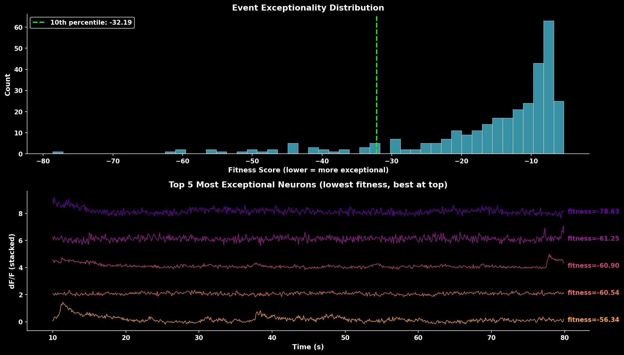
Event exceptionality analysis. The fitness score distribution shows most neurons have moderate exceptionality. Lower fitness scores indicate neurons with rarer, more exceptional events. The trace panel shows the 5 most exceptional neurons (lowest fitness scores) with best-quality neurons displayed at top.

---

Loading Results

Load Planar Results

Load all Suite2p outputs from a plane directory:

from lbm_suite2p_python import load_planar_results

results = load_planar_results("path/to/plane01")
# or
results = load_planar_results("path/to/plane01/ops.npy")

# Access data
F = results['F']           # (n_rois, n_frames) fluorescence
Fneu = results['Fneu']     # (n_rois, n_frames) neuropil
spks = results['spks']     # (n_rois, n_frames) deconvolved spikes
stat = results['stat']     # ROI statistics array
iscell = results['iscell'] # (n_rois, 2) classification

# Filter for accepted cells
iscell_mask = iscell[:, 0].astype(bool)
F_cells = F[iscell_mask]

Load Ops

Simple utility to load ops.npy:

from lbm_suite2p_python import load_ops

ops = load_ops("path/to/ops.npy")
# or
ops = load_ops("path/to/plane01")  # auto-finds ops.npy

Load Traces (Accepted Only)

Load only accepted cell traces:

from lbm_suite2p_python.postprocessing import load_traces

F, Fneu, spks = load_traces(ops)
# Returns only traces where iscell[:, 0] == True

---

Export Utilities

Ops to JSON

Export ops dictionary to JSON for reproducibility:

from lbm_suite2p_python.postprocessing import ops_to_json

# From ops.npy file
ops_to_json("path/to/ops.npy", outpath="ops.json")

# From dictionary
ops_to_json(ops_dict, outpath="ops.json")

---

Complete Workflow Example

import lbm_suite2p_python as lsp
import numpy as np

# Load results
results = lsp.load_planar_results("path/to/plane01")
ops = lsp.load_ops("path/to/plane01")

F = results['F']
Fneu = results['Fneu']
stat = results['stat']
iscell = results['iscell']
fs = ops.get('fs', 30.0)

# 1. Apply ROI filters
from lbm_suite2p_python.postprocessing import (
    filter_by_diameter, filter_by_area, filter_by_eccentricity
)

iscell_mask = iscell[:, 0].astype(bool)
iscell_mask = filter_by_diameter(iscell_mask, stat, ops)
iscell_mask = filter_by_area(iscell_mask, stat)
iscell_mask = filter_by_eccentricity(iscell_mask, stat)

# 2. Filter arrays
F_filt = F[iscell_mask]
Fneu_filt = Fneu[iscell_mask]
stat_filt = stat[iscell_mask]

# 3. Calculate dF/F
dff = lsp.dff_rolling_percentile(
    F_filt - 0.7 * Fneu_filt,
    tau=1.0, fs=fs
)

# 4. Estimate noise quality
noise = lsp.dff_shot_noise(dff, fs)
print(f"Median noise: {np.median(noise):.3f} %/√Hz")

# 5. Sort by quality
F_sorted, sort_idx, quality = lsp.sort_traces_by_quality(
    F_filt, Fneu_filt, stat_filt, fs
)

# 6. Visualize top neurons
lsp.plot_traces(
    F_sorted[:20],
    fps=fs,
    title="Top 20 Neurons by Quality"
)